Permutations
Combinations
Probability
Random Variables and Probability Distributions:
One of the key uses of statistics is to deal with uncertainty. Statistics can assign probabilities to uncertain events, allowing us to have some confidence as to the outcome. In many cases it is desirable, even necessary, to know all the possibilities before assigning probabilities. One method of determining the possibilities is counting outcomes. This can be a laborious task for complex problems but, fortunately, we can use tree diagrams to aid in this endeavor.
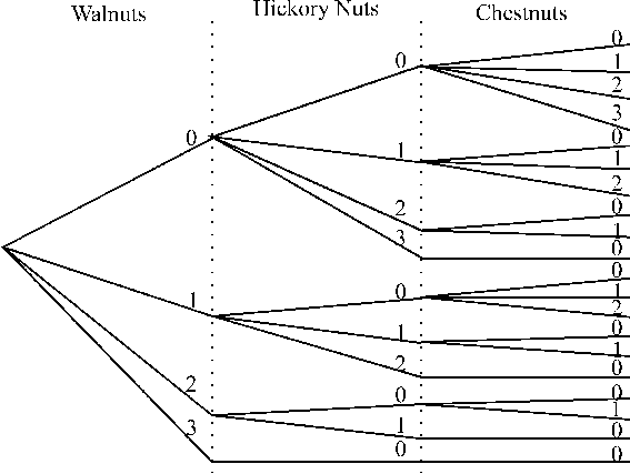
To see how a tree diagram works, think of a squirrel in an experiment. A squirrel can only carry three nuts back to its nest at one time, and there are four types of nuts (walnut, hickory nut, chestnut, and pecan) that have been distributed evenly and randomly in the study area. What are all the different ways that the squirrel can pick nuts to take back to its tree? We set up the tree diagram with three levels of decisions (say walnut, hickory nut and chestnut). We don't need to account for pecans as a decision because it is the default choice if the others are not taken. On the left of our tree diagram we make branches for each of the possible decisions regarding walnuts: the squirrel could choose zero, one, two, or three walnuts. If zero walnuts are chosen, then the squirrel can choose zero, one, two, or three hickory nuts. However, if one walnut is chosen, then it can choose zero, one, or two hickory nuts, because it can only carry three back to the nest. This process is continued until all possibilities can be accounted for by branches in the tree. Then, one can count the branches at the end of three and this will be the number of possibilities. In this case, there are 20 possible ways the squirrel could gather its dinner:

Now imagine what the problem would be like if there were 10 types of nuts and the squirrel could carry four at a time. As you can see, tree diagrams would be difficult to use for many types of problems. However, there are some rules that allow us to determine the number of possibilities for many types of problems without actually counting them.
The multiplication of choices rule says that if we make choices in two steps and the choices are independent of each other, then the total number of choices is the product of the individual choices. For example, say the same squirrel could carry one nut and one fruit back to its tree. If there are four nuts and three fruits then there are 4*3 = 12 possibilities. However, the second choice can not depend on the first. For that reason, this approach can't be applied to the "10 nuts carried four at a time" problem.
The multiplication rule can be extended to any number of choices. Say there are k choices to be made by the squirrel, and the number of possibilities for any choice is n1 , n2 ,... nk. So lets say the squirrel can choose one of 4 nuts, one of three fruits, and 1 of ten seeds. The number of possibilities is now 4*3*10 = 120. This is much easier than counting, but each decision must be independent of each other, and only one choice can be made from each category. Problems like "10 nuts carried four at a time" are most easily done by counting, but we now use computers to do the laborious part for us.
An extension of the multiplication rule can be applied to several choices from the same set of data when the order of the choices is important. For example, assume that the squirrel has 10 nuts to choose from, but he can only carry two. What are the possible ways he can choose the two nuts? We know that the squirrel has 10 nuts for the first choice and 9 for the second. The number of possibilities is 10*9 = 90. This is an example of sampling from a population with removal, and we call the choices permutations. Permutations can be applied when a subset objects are chosen from a equal or larger set of unique objects when the order of choices matter. Permutations consist of a series of numbers, each one unit less than the last, multiplied together. When this series extends down to one it is a factorial (n !). For example, the product 3*2*1 is 3! ("three factorial"). By convention 0! is assigned a value of 1.
With factorials we can develop a mathematical expression for
the number of permutations. The series of multiplications used
to apply the multiplication rule to permutations is a portion
of a factorial. If we have a set of n objects from which
we choose r , then the number of permutations ![]() can
be expressed as:
can
be expressed as:

So, our example of 10 nuts of which the squirrel can choose 2 is given by:

The first formula is easier to perform by hand because it requires fewer steps, but the second one is easier to remember. The second formula also has the advantage that it can be used to determine the number of possibilities of zero objects taken from a set of n :
Also, with calculators having a factorial function, the second expression is not more laborious to calculate than the first. One final note on permutations deals with r = n. This is a complete factorial of n, which can be seen from:
which can get extremely large very rapidly. For example, 5! = 120, 10! = 3628800, and 15! = 1.31 x 10¹². Most pocket calculators can't handle numbers of 1099 or larger, i.e., factorials beyond 69!.
With permutations, we are interested in the order in which objects are chosen, but sometimes we may not be interested in this at all. For example, our squirrel may be presented with three types of nuts to choose from. He could chose a walnut first, then a hickory nut, and finally a chestnut. The order in which the nuts were chosen would be different, but the combination of nuts chosen would be the same. would be different from choosing a hickory nut, a walnut and a chestnut. Sometimes, we may only want to know what items from a set can be chosen. Of the four types of nuts in the first example we could get the following combinations of three things:
| Walnut | Hickory Nut | Chestnut |
| Walnut | Hickory Nut | Pecan |
| Walnut | Chestnut | Pecan |
| Chestnut | Hickory Nut | Pecan |
The formula for the number of combinations of n objects taken r at a time is:

There are two ways that combinations are often presented in
notational form; ![]() . You should be
familiar with both. Sometimes these are referred to as binomial
coefficients, which are used extensively in genetics.
. You should be
familiar with both. Sometimes these are referred to as binomial
coefficients, which are used extensively in genetics.
As with the formulae for permutations, the first one for combinations is easier to calculate by hand, but the second is easier to remember. The second can also handle the situation where the number chosen is 0:
So, how may combinations of 20 food items can the squirrel take four at a time?
As you can see, one can simplify many problems by applying
arithmetic rules. This is particularly beneficial when dealing
with large factorials like that couldn't be handled by calculators.
There is another "trick" that one can use with combinations.
If we want to know the number of combinations of choosing 16 things
from 20 we can also reword that as the combinations of not choosing
4 things from the 20. That means ![]() or
or
![]() . This is the rule of binomial
coefficients, which states that there just as many combinations
of choosing r objects from n as there are of leaving
n - r objects. For example, try to solve
. This is the rule of binomial
coefficients, which states that there just as many combinations
of choosing r objects from n as there are of leaving
n - r objects. For example, try to solve ![]() with
your calculator without using the rule of binomial coefficients.
It is a rather simple matter to look for the combinations of 2
items left out of the 100:
with
your calculator without using the rule of binomial coefficients.
It is a rather simple matter to look for the combinations of 2
items left out of the 100:
Now that we can determine the number of possible outcomes, we can begin to assess their probabilities. The most simple concept in probability deals with successes and failures. Simply stated, if there are n equally likely possibilities of which one must occur, and s are regarded as a success, then the probability of the success is s /n.. This rule has little application in biostatistics, because so few things have equal possibilities, but it can be extended to random processes which approximate some natural phenomena. For example, assume that there are 50 genes at a given locus in a population. Of these 50, five of the genes are lethal and a biologist samples 2 individuals (2 genes per individual = 4 genes). What is the probability that one and only one of the lethal genes will be in the sample. First of all, we need to know how many ways we can sample the four genes, regardless of order. This is the combination:
In this case a successful outcome would be finding 1 lethal and 3 normal genes in the two individuals. The number of combinations that meet this criteria are:
So, the probability of finding one and only one lethal gene in two individuals sampled is:
which is a 21% probability, or better than 1 in 5 odds.
This simple rule of probability works fine when all outcomes are equally likely, but what happens when some are more likely than others. When this is the case, we must rely upon frequency interpretation, which states that the probability of an event is proportional to the frequency of that event happening over long sampling periods. For example, if a biologist watches a bird feed 100 times, and 62 of those times it eats thistle seeds, then the frequency of eating thistle seeds is 62/100 = 62%. The frequency interpretation would suggest that the next time the bird feeds, there will be a 62% probability that it will eat thistle. Of course, how good an estimate this probability is depends on the sample (among other things), and 100 foraging periods may not adequately represent the bird's true behavior (the observations may all have occurred in the summer when thistle is abundant). Furthermore, these probabilities are limited to only that bird; applying them to other birds is termed extrapolation. As we shall see in future lectures, extrapolation is a dangerous path to take in biostatistics.
When biologists conduct experiments or take samples from nature the generate values that can be manipulated and analyzed statistically. We call these values random variables. Random variables can take on different values that all must occur within a sample space. For example, if a researcher uses 40 plants in an experiment he/she cannot obtain a result like "46 produced seed in the first six months of the experiment." There are two types of random variables: those that consist of integer values which are called discrete (e.g., the number of "teeth" in the sawtoothed edge of a leaf, the number of eggs laid by a lizard (clutch size), or the number of colonies of bacteria on a Petri dish), and those that can take only be any whole number within a range, which are called continuous (e.g., the length of the perimeter of a leaf, the mass of a lizard's clutch of eggs, or the area of a Petri dish covered by colonies of bacteria).
The outcomes of an experiment, or the random variables, can have probabilities associated with them. The distributions of these probabilities are called a probability distribution. For example, our wildlife biologist believes that raccoons usually require at least one hour to find their first meal after weaning. One way to test this hypothesis is to construct a frequency distribution of his observations of the 20 raccoons. This produces the following graph:
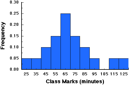
which looks much like the histograms we developed for distributions in earlier lectures. Examination of this graph reveals that 65 percent (0.65 * the total number of raccoons) required one or more hours to find their first meal, while only 35 percent (0.35 * the total number of raccoons) required less than one hour.
As with everything in statistics, we have some rules regarding probability distributions:
1. Values must be in the range from 0 to 1, inclusive
2. The sum of all values must be 1
Ideally, we would like to have a mathematical function that describes the probability distribution, but this may not always be possible. In the above example, it would be hard to develop an expression that gave exact values for the probabilities. However, there are cases when this is possible. Take the case where there is a sample space of 5 elements, each with an equal probability of occurring. The probability of obtaining any element in a sample would be f(x) = 1/5. Thus, the probability of drawing element 1 from the sample space (f(1) = 0.2) is the same as drawing element 3 (f(3) = 0.2). Such functions can be quite complex, but the also can make our lives easier. When we perform statistics on a data set we usually assume that it possess some underlying distribution. In the following sections we will cover many of the distributions used in statistics and see how they can be expressed mathematically. Expressing probability distributions as functions also as the benefit of allowing the statistician to check and see if the probabilities sum to 1 (rule 2).
Many of the examples we have used so far amount to asking the question "how many successes will we have in a given number of trials?" When we address problems of this nature, we are assuming three things:
1. The number of trials is a fixed number
2. The probability of a success (or failure) is the same for each trial
3. Each trial is independent of all the others.
The multiplication rule of probability allows us to determine the probability of events occurring when they are independent. If we let p represent the probability of a success (1-p is the probability of a failure), then for x trials we would simply multiply p times itself x times, or simply raise p to the power of x (px). We must also have failures taken into account, however, whenever we want to know the probability that there will be some specific number of successes and failures (which is what a probability distribution tells us). If there are n trials, then the probability of failures is given by (1-p )n-x. The probability of finding exactly x successes and n-x failures in out of n trials in a specific order is then given by:
However, this probability applies to any element in the sample space that consists of x success and n-x failures. We are interested in all such points, so we must account for all the combinations in which this result can be obtained. The probability of getting x successes in n independent trials is given by the binomial probability distribution:
Below is a graph of the binomial distribution for 5 trials:
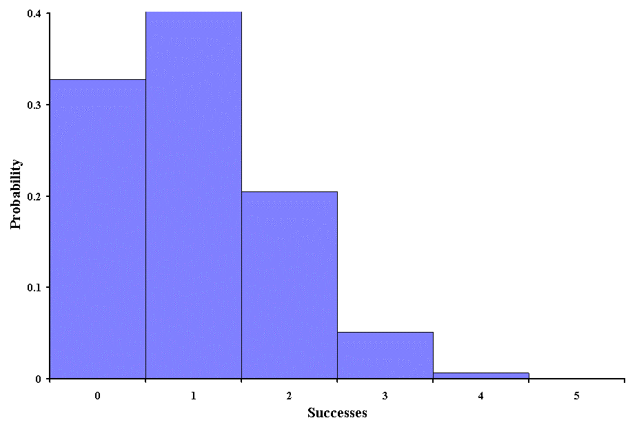
From such a graph it is easy to see that the probability of obtaining 4 or 5 success is very unlikely. When events are equally likely we can use a binomial distribution because p is a constant (in this case p = 1/5). Such probabilities are not always obtained in biostatistics, but the binomial distribution is widely used in genetics.
Beyond determining the probability of a certain number of success, we may also be interested in how many trials it would take to achieve a success given a certain sample space. From the binomial distribution we can make some modifications to determine the probability that first success will occur on a given trial (x ). This is called the geometric probability distribution, and it is expressed as:
The modification involves a bit of logic. If the success occurs on the x th trial, then it must have been proceeded by x -1 failures. Additionally, it is the first success, so we raise p to the first power. Although this is not widely used in biostatistics, it does have some use. Consider the following problem. A biologist wants to catch an albino monkey, but they are very rare in the population studied (1 in 200 or p = 0.005). If the researcher can only catch one animal per day, and there are only 10 more days before he must return to the university, what is the probability of catching an albino monkey on each of the days? The following graph shows the probabilities:
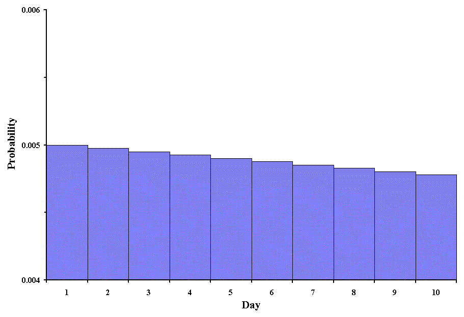
It would appear this researcher has a problem. Not only is it very unlikely that an albino monkey will be caught, but the probability decreases each successive day! The researcher might better spend the time doing something else.
When discussing the multiplication rule, we introduced the concepts of sampling with and without replacement. Sampling with replacement means that once an element is selected from the sample space, it is replaced so that it is available in future selections. The binomial distribution applies only for sampling with replacement. As an example, imagine a researcher that needs 4 mice for an experiment and there are 20 in the laboratory. Of these, half are brown and the others are white (p = 1-p =0.5). What is the probability that the researcher will choose 3 white mice? With the binomial, we would find the solution as follows:
but the probabilities of obtaining a white mouse change each
time a subject is chosen. Before the first selection, the probability
of obtaining a white mouse is 10/20 = 0.5, and before the second
selection (if a white mouse is chosen) it is 9/19 = 0.47. Thus,
we can't use the binomial distribution to determine the probability.
Instead, we must recognize that there are ![]() ways
of obtaining three mice from the sample space, and
ways
of obtaining three mice from the sample space, and ![]() ways
of obtaining three mice from the white group. From the classical
rule of probability (s/n) we can see that the probability is
ways
of obtaining three mice from the white group. From the classical
rule of probability (s/n) we can see that the probability is ![]() , which is much greater than
expected from the binomial.
, which is much greater than
expected from the binomial.
To generalize, lets assume that a represents the set
of successes and b represents the set of failures. If we
choose n objects, what is the probability of obtaining
x successes? We know that n objects can be sampled
from the entire sample space (a+b) in ![]() ways,
that x of the successes can be chosen from the set of successes
in
ways,
that x of the successes can be chosen from the set of successes
in ![]() ways, and that n-x
failures can be chosen from the set of failures in
ways, and that n-x
failures can be chosen from the set of failures in ![]() ways.
So, when sampling without replacement, the probability of getting
x successes in n trials is:
ways.
So, when sampling without replacement, the probability of getting
x successes in n trials is:

which is the hypergeometric probability distribution.
In our previous discussions of probability, we have assumed
that all the sample spaces are finite in size (the third postulate
of probability). In fact, we can handle problems that are infinite
as long as they consist of the whole numbers (i.e., 0, 1, 2, 3,
... ). In this case, we simply restate the third postulate such
that ![]() . When the number of trials
(n ) is very large and the probability of success (p
) is very small. When this is the case, we can use an approximation
of the binomial distribution:
. When the number of trials
(n ) is very large and the probability of success (p
) is very small. When this is the case, we can use an approximation
of the binomial distribution:
which is called the Poisson probability distribution. The natural exponent (e ) is approximately 2.718. In general, we won't use this to approximate the binomial, because the binomial is so easy to calculate with modern calculators and computers. However, the Poisson distribution has some interesting uses in biology. As we will see, one can use np to estimate the mean number of successes, so the formula can be rewritten as:
You will see this formula in many ecology texts as an approximation to a random distribution. Thus, we can compare sample distributions to the Poisson to determine the likelihood they are random.This distribution also has application in analyzing the radioactivity of very low activity radiaion sources.
Last Updated: Friday, 3 January 2003, 1:00 PM