Hypothesis Testing
Tests of Significance
One-sample Test of Means
Two-sample Test of Means
Paired Data
Of course, we often want to say more than what the range of
likely values for the population mean is. It is often desirable
to ask the question of whether the sample mean is different from
a given population mean. This is one way we can determine the
likelihood that a sample came from a particular mean. For example,
we may know that the average male widow bird has a tail length
of 0.85m. If we took a sample from a newly discovered group of
widow birds, we would like to know if the new population has a
similar distribution as the previously known population. The mean
is a descriptor of the population, so we could test to
see if the sample mean was significantly different from
0.85. When we do this, we are hypothesizing about the population
mean of the new group. In hypothesis testing, we formulate comparison
between a null hypothesis and an alternative hypothesis.
We want the alternative hypothesis to be one that can be addressed
without rules of probability. It is difficult to determine the
probability that a mean will be some amount greater than or less
than another value. For example, how would you determine the probability
that the new group has a mean that is between 4 and 5 times that
of the old mean? It is possible, but it leaves open the question
of what happens when the new group mean is actually 5.1 or 3.9
time greater. We usually formulate the null hypothesis in such
a way that it can be rejected with some certainty that is easily
defined with a probability statement or confidence interval. As
a rule of thumb, we say that the null hypothesis must contain
the equal sign. We may have a null hypothesis that says the new
mean is equal to (=), less than or equal (![]() ) or greater
than or equal to (
) or greater
than or equal to (![]() ) the old
mean. If we can reject such an hypothesis, we may state with some
confidence the alternative hypothesis is true. The null and alternative
hypothesis will look like this:
) the old
mean. If we can reject such an hypothesis, we may state with some
confidence the alternative hypothesis is true. The null and alternative
hypothesis will look like this:
|
|
|
|
|
|
|
|
|
|
|
|
So, when we frame our questions, we often use the alternative hypothesis to express the relationships we are really looking for.
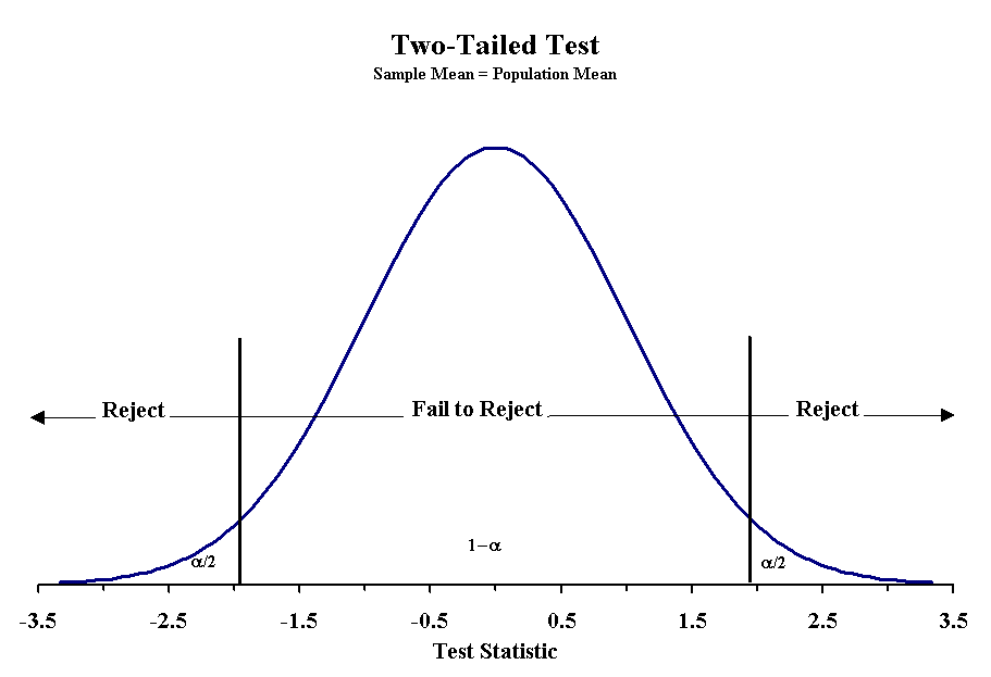
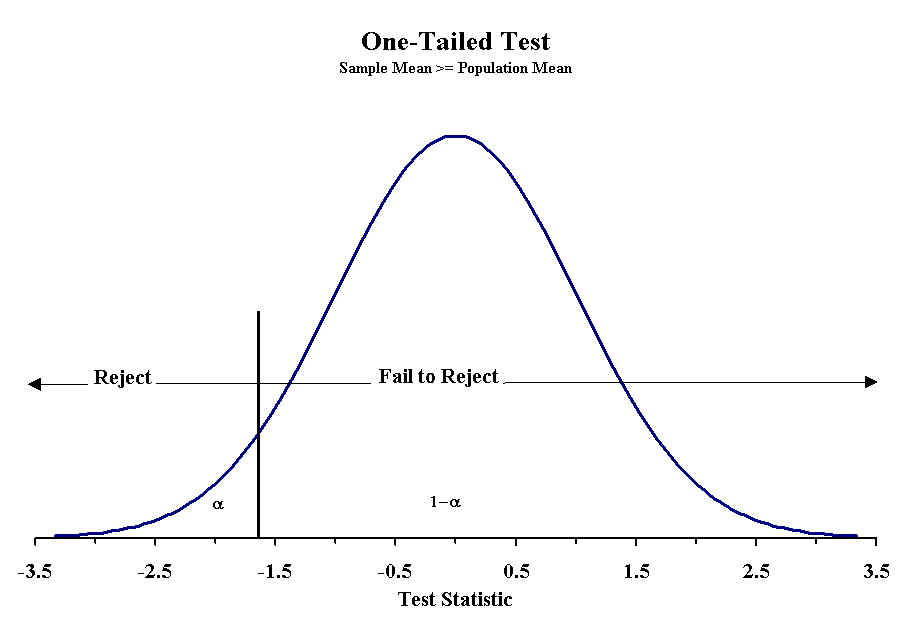
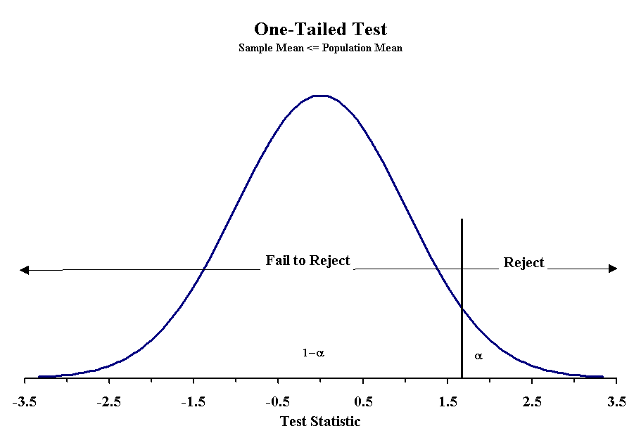
When designing the hypotheses, we must recognize how they affect the determination of probability. We have already seen cases when we were uninterested in which side we err, and this is called a two-tailed probability. When the null hypothesis uses the equals sign, we are dealing with a two-tailed probability. For the other null hypotheses, we use a one-tailed probability. This greatly affects or determination of the appropriate z or t-score to use. When we use a two-tailed probability then the confidence interval is set by - zα/2 and zα/2. With one-tailed statements, it will be either -zα or zα.
When we test any hypothesis, we are interested in the values that will lead us to reject the null hypothesis. This is different from saying that we accept the alternative hypothesis! This distinction is vitally important, and is the major strength of science as a way of thinking: we can never absolutely prove that any particular hypothesis is correct! With additional information, we may later frame our alternative hypothesis as the null hypothesis for a completely different alternative hypothesis! This allows science to "self-correct" itself when accepted hypotheses later prove to be false.
With the two-tailed test, we reject the null hypothesis when sample mean is either too large or too small. We determine this degree of difference by the value of the z-score or t -score associated with our confidence limits. The same is true for one-tailed test, but the limits are only on one side of the normal distribution. In all cases, the area not explained by the null hypothesis must equal α.
When we deal with hypothesis testing there are many possible outcomes. If the null hypothesis is true, and we fail to reject, then we have made a correct decision. The same is true if the null hypothesis is false and we reject it. However, it is possible to make an error. The null hypothesis may be true, but we reject it anyway. This is a Type I error. The hypothesis may also be false and we may fail to reject it. This is a Type II error. The probability of committing a Type one error is α. In other words, the probability statement we make reflects our willingness to reject the null hypothesis even if it is true. Smaller values for α mean less willingness to make a Type I error. The probability of committing a Type II error is usually denoted with β. This is often represented as a power statement (as opposed to probability statement), because it reflects our power of exposing a false null hypothesis. Ideally, one would like to balance the probabilities of committing each Type of error. In practice, however, it is often difficult to determine the power of a statistical test, and it is beyond the scope of this class. In general we are satisfied with β = 0.1.
When testing hypotheses, we must proceed in a particular fashion if we are to achieve our desired goals. Generally, we follow the following steps:
The third step depends on the sampling distribution of the sample statistic. In the case of the mean, we can assume the sampling distribution approximates the normal distribution (or t distribution). We must also determine whether the probability of Type I error is distributed across both tails of the distribution or just one. Step four requires that we relate the sample statistic to the hypothesized parameter in a manner that allows us to assess the probability of a Type I error. When the value of the test statistic falls outside the probability associated with the null hypothesis we fail to reject the null hypothesis.
Note: The first step is the most difficult part of doing science, and the failure to correctly state the problem in terms of a single "either-or" set of outcomes is the most common cause of failure in scientific research. The third, fourth, and fifth steps can also lead to failure, but in most cases, the problem is that the experiment is designed properly, but the hypothesis is wrong!
Of course, the test statistic depends on several factors. For the mean, we have seen a few already, we just discussed them under a different framework. Sample size is important for determining the appropriate test statistic, but so are things like the standard deviation. We will cover several test statistics in the next few lectures.
Making the decision to reject the null hypothesis requires one to know the probability of obtaining a particular value of the test statistic given an underlying distribution. For much of what we have seen so far, we have used a normal distribution and obtained the z-score associated with a probability. This basic approach can be used for any statistical test. Below are three figures that show the critical values for rejecting the null hypothesis with a 5% probability of Type I error.


When using a normal distribution the critical values for each Type of test with probabilities of Type I errors of 5% and 1% are given below:
|
|
|
|
|
|
|
|
|
|
|
|
|
|
|
|
When using a t-distribution we have to determine the critical values based on the degrees of freedom.
When performing a one-sample test we often are trying to determine if the sample mean has a particular relationship to a hypothesized population mean. In that case we can simply standardize the sample mean given the appropriate distribution. For large samples the appropriate distribution is the normal, and for the
Let's imagine you are interested in reproduction of oak trees. You have a very large population of oaks and you believe the mean number of acorns produced by a tree is 500. When performing the test we must follow the rules listed above. First we formulate our hypotheses. In this case we are interested in determining if the sample mean is equal to the hypothesized mean. Our hypotheses can be stated as:
H0: Sample Mean = 500; Hα: Sample Mean <> 500.
Now we must specify the maximum probability of a Type I error. In this case you want to be 95% sure of your conclusion, so the Type I error is 0.05. Next we must determine the appropriate test criterion. We know that the sample mean should be normally distributed if we take a large sample size. We can determine the z-score for our sample mean with the following formula:
This is our test statistic. We must take a sample and calculate the value of z to determine the significance of the test. Let's say you sample 35 trees and obtain a mean number of acorns of 621 and a standard deviation of 152. The test statistic would be:
Because we have a two-tailed test, we must reject the null hypothesis if our test statistic is greater than 1.96 or less than -1.96. In this case we can reject the null hypothesis. We cannot say that the sample mean is greater than the hypothesized value (even though our results would suggest it is) because we only tested to see if they were equal. If we had formulated our hypotheses as:
H0: Sample Mean <= 500; Hα: Sample Mean > 500.
We could have used a one-tailed test with a critical value of 1.65. As you see, our test statistic is greater than this critical value, so we could have reject this null hypothesis as well. However, we cannot reformulate our hypotheses after we have collected the data. We must start from the beginning and completely redo the problem, including obtaining a new sample, if we don't want to artificially change the probability of a Type I error. This is a common problem in statistics, where the same hypothesis is repeatedly tested. The real probability of rejecting the null when it is true increases with each test of a hypothesis. To avoid this we must obtain a new sample and reformulate or hypothesis. There are some statistical means of correcting for such problems, such as the Bonferroni and Sequential Bonferroni corrections. However, these corrections result in diminished power (greater Type II error). We will discuss some of these issues in the section on experimental design.
When working with a small sample the sample means follow a t-distribution. For that reason, we must use a different test statistic:
and we must know the degrees of freedom. If we use our same example with the oak trees and obtain a sample of 20 trees, our degrees of freedom are 20-1 = 19. Using a two-tailed test we see that the critical values of t are -2.09 and 2.09. Our test statistic is:
so we can safely say that the sample mean is not equal to the hypothesized value of 500.
Sometimes it is necessary to determine the relationship between two sample means. For example, can we safely say that two samples with means of 5.3 and 3.9 came from the same population? To do this, we must modify our test statistics slightly. One thing we must recognize is that each sample will have a standard error associated with its mean, because neither is likely to be exactly the same as the population mean. Another question we may be interested in is determining if two sample means differ by a set amount. In that case, we will also need to account for the fact that neither sample mean reflect the true mean of the population it comes from (i.e., there are errors in the estimates). Because variances are additive, we can compute a standard error for the difference between means. To do this we take our standard errors, square them so they are now measures of variance, add them together and take the square root:
This new standard error can be used to test hypotheses concerning two sample means. We have two Types of questions: 1) do the samples differ (are they from the same population), or 2) do they differ by a set amount. If we let δ represent the hypothesized difference, we can see that the following treatment of the means will satisfy both questions:
When δ = 0 then we are asking the first question. When δ <> 0, then we are asking the second question. We need only to set δ equal to the hypothesized difference.
For large sample the difference between two means is normally distributed. Our test statistic becomes:

As an example, let us consider two researchers that claim that the mean number of times that a patient requires antibiotics after heart surgery are 1.7 and 3.2. The first study was based on a sample of 52 patients and had a standard deviation of 0.87. The second study had a standard deviation of 1.57 and was based on 32 patients. Are the two samples statistically different at 95% confidence level?
In this case δ = 0 and our hypotheses would be:
H0: μ 1 - μ 2 = 0, Hα: μ 1 - μ2 <> 0
The probability of a Type I error is 0.05, and our test statistic is

We use the same rejection criterion as for the single-sample test, so we can safely say that these samples do differ. What would we do if the first research claimed that the other hospital had at least 1.5 more infections per person following heart surgery (perhaps claiming their hospital is better)? We could reframe the hypotheses and make it a one-tailed test:
H0: μ 2 - μ 1 >= 1.5, Hα: μ 2 - μ1 < 1.5
Our test statistic would be:

We can't support this researcher's claim, because our test statistic is less than the critical value of 1.65.
When dealing with small samples, the computation of the test statistic is more complex. In this case, the test statistic is sampled from a t-distribution and our formula for the standard error becomes more complex. Because of the bias in the estimator of the standard deviation, we must calculated a pooled standard deviation before determining the standard error:
and the standard error becomes:
Our test statistic becomes:

having a t-distribution with n1+n2-2 df
When using this last test it is important to recognize that there is an assumption that the population standard deviations are not significantly different from each other. We will see in the next lecture how to test for such a significance, but for now one must recognize that unequal variances require the use of the normal approximation given by z above.
At times sample sizes may prevent the use of the normal approximation. In cases where sample sizes are small and variances are different we can use the Behrens-Fisher approximation to the t-distribution. This is the same test statistic as for the normal distribution, but the degrees of freedom are given by:

This is a fairly complicated computation (although again, not really so on a modern computer), which explains why it is rarely used. But, it SHOULD be if the circumstances warrant it.
Many Types of data allow the researcher to pair observations. For example, one may be interested in determining if the first born of a set of twins grows to be taller. We can pair the observations from the first sample (first born) with observations in the second sample (last born). This is not really a problem for statistical analysis. We can simple subtract the observations in the second sample from those in the first and produce a new random variable (δ). The mean of this random variable is sampled from a normal (large n) or t-distribution (small n). For that reason we can use the standard one-sample tests as outlined above. The only thing that has changed is we use the mean and standard deviation of δ and we frame our hypotheses accordingly. As an example, we will test the null hypothesis that the difference between our twins is 0 with the following data.
|
|
|
|
|
|
|
|
|
|
|
|
|
|
|
|
|
|
|
|
|
|
|
|
|
|
|
|
|
|
|
|
In this case the mean difference is zero, the standard deviation is 0.58 and t = 0. We can not reject the null hypothesis that δ = 0, so it would appear that twins grow to the same height.