Estimating the Variance
and Standard Deviation
Single Sample Tests: Small and Large Sample Sizes
Two Sample Tests
Smith's Test
Estimation of Proportions
Tests of Proportions: Single Sample
and Two Sample Tests
χ2 (Chi-square): Contingency
Tables and
Goodness-of -Fit
We have seen that there is a bias in the variance standard deviation, which required us to apply a small correction factor. We have also seen the variance is of a different scale than the mean. There is another difference between the sample mean and variance, these statistics have different sampling distributions. While all combinations of sample means from a population have a normal distribution, sample variances have a chi-square (χ2 ) distribution. We standardize our sample deviations to this distribution with the following formula:
Like the t-distribution, this distribution changes with
the degrees of freedom (n - 1). This distribution consists
of all the real numbers greater than or equal to zero. Unlike
the normal and t-distributions, the χ2 is not symmetrical.
This means that ![]() , so we have to be more careful when determining
our probabilities of different outcomes.
, so we have to be more careful when determining
our probabilities of different outcomes.
This lack of symmetry is readily seen from the confidence intervals for the variance. We can say with 95% confidence that our standardized variance lies within the range of:

With a little algebra, we can solve for the parameter in question and determine the confidence interval:
For α = 0.05 and 20 df we find that ![]() and
and ![]() . With a sample variance of
3, we get confidence limits of 1.756 and 6.256. This confidence
interval has a range of 4.5 and a median of 4.006. The median
of the interval is shifted to the left of the sample variance,
which was not the case for the normal and t-distributions.
. With a sample variance of
3, we get confidence limits of 1.756 and 6.256. This confidence
interval has a range of 4.5 and a median of 4.006. The median
of the interval is shifted to the left of the sample variance,
which was not the case for the normal and t-distributions.
The confidence interval for the sample standard deviation can be obtained by taking the square-root of each side:

which gives us 1.325 and 2.501 with the example above.
The above formulas for confidence intervals are designed for
small sample sizes. As sample sizes get larger (n >=
30), the sampling distribution of the statistic takes on an approximately
normal distribution with a standard deviation of ![]() . Thus, for large sample sizes,
we can standardize the statistic to a normal distribution with
the following confidence intervals:
. Thus, for large sample sizes,
we can standardize the statistic to a normal distribution with
the following confidence intervals:

Using the same example, but with a sample size of 40, we get confidence intervals of 1.421 and 2.218. Again, this is not a symmetrical distribution.
We are often interested in determining how a sample variance is related to a hypothesized value. This involves the same sort of probability statement that we used for the single-sample test of means. In the case of the variance, we use the chi-square distribution for small sample sizes and the z distribution for large samples. Unlike our tests of sample means, the following tests are very sensitive to the assumption that the sample and population have a normal distribution. This is not the same as assuming that the statistic will be normally distributed. For that reason, testing of variances is fraught with problems.
The test statistic for small samples is:
where σ2 is the hypothesized value of the variance. We determine the critical values from a table using n-1 degrees of freedom. The following table shows the criteria for rejecting different null hypotheses (H0):
|
|
|
|
|
|
|
|
|
|
|
|
When sample sizes are large, the sampling distribution of the standard deviation is approximately normal, and we use the test statistic:
Note that we use the hypothesized value to also estimate the standard error. This uses the same rejection criteria as the large-sample test for means.
When testing two sample means, we were able to use the z distribution because each had a sample distribution that was approximately normal. This is not the case for variances. In fact, variances don't have a chi-square distribution, either. In the case of two samples, we must use the F distribution and test the ratio of the variances, not their differences. This distribution has two different degrees for freedom (n1-1 and n2-1). The test statistic is of the form:
and we determine which variance to call ![]() depending upon our null hypothesis.
depending upon our null hypothesis.
|
|
|
|
|
|
|
|
|
|
|
|
|
|
|
|
|
|
|
|
When looking up the critical values in a table, we use the degrees of freedom for the numerator first and degrees of freedom for denominator second.
As has been mentioned repeatedly, the standard test statistics for the standard deviation and variance are very sensitive to the assumption of normality of both the population and the sample. It is not always possible to meet these criteria, or even to determine whether the criteria can be met. Smith's test is distribution free and can be applied to any data set. Instead of relying solely upon the standard error of an estimate (standard deviation of the sample estimates), it uses the variance. The variance of the variance is given by:

One can calculate the variance of the estimator for any number (k) of populations and the test statistic will have chi-square distribution with k - 1 degrees of freedom. The test statistic is given by:
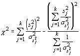
Although this is a rather complicated formulation, with modern computers this shortcoming is small compared to the great gain in versatility. Additionally, it can be used for any statistic for which a standard error can be calculated. Thus, it is a true test of homogeneity of variance: you need only replace the sample statistic s2 with another statistic. For example, if you suspect that the means of two populations differ, and wish to determine if the dispersion also differs, you could use the coefficient of variation:
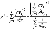
Because it can be used for any number of populations, we can substitute it for analysis of variance, which we will see later can only determine differences in variances when means are equal (without standardization).
If there are x outcomes in an event from a sample space with n outcomes, then the proportion of sample space represented by the events is defined as:
This can be used as a point estimate of the population proportion, just as a mean represents a point estimate of central tendency. Unlike the mean, when we discuss proportions,we are usually dealing with successes in a set of independent trials. As we saw in the section on the rules of probability, p represents the probability of obtaining a success.
In order to determine how adequate our sample proportion represents
the true population proportion (or probability of obtaining a
success), we must determine its sampling distribution. The sampling
distribution for a proportion is approximately binomial with a
mean of ![]() and a standard deviation of
and a standard deviation of ![]() . To avoid confusion between
statistics and parameters, we generally use p to represent
the population parameter, and x/n or
. To avoid confusion between
statistics and parameters, we generally use p to represent
the population parameter, and x/n or ![]() to represent the sample statistics.
Using this representation, the statistics are:
to represent the sample statistics.
Using this representation, the statistics are:
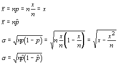
One could use either formula, but the latter formulae allow the interpretation of summary data that don't include the number of successes (x).
You can use the mean and standard deviation to standardize the sample:
which has approximately a normal distribution when np and n(1 - p) are greater than about 5. From this, we can determine the probability of falling within two critical values in the distribution. We need only perform some "simple" algebra:
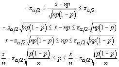
Unfortunately, we have the parameter we are interested in estimating on each side of the inequalities. As we did with the standard deviation in other tests, we must estimate the population proportion with the sample proportion. The confidence interval for the proportion is given by:
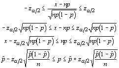
The expression ![]() is the standard deviation of
the sample space, or the standard error. This error can be used
to determine the maximum error of the estimator with:
is the standard deviation of
the sample space, or the standard error. This error can be used
to determine the maximum error of the estimator with:
which can be used to determine the minimum sample size necessary to obtain a desirable error (1 - α). If you already have an estimate of the proportion, you can simply rearrange the equation to yield:
However, you often don't have an estimate of the proportion, so to be conservative, you can use:
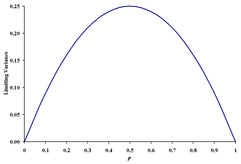
This expression is very conservative, because it uses assumes
maximum variability in the population. The quantity ![]() is termed the limiting variance,
and it is maximized when p = 1 - p = 0.5, as you can
see in the following figure.
is termed the limiting variance,
and it is maximized when p = 1 - p = 0.5, as you can
see in the following figure.
By assuming the variance is at its maximum value, one decreases the probability of making an error of inference, but one also may waste time and money obtaining a large sample. For example, if one wanted to be 95% confident in the estimation of the population proportion, one would require a sample size of 384 if we don't want to be off by more than 0.05. On the other hand, if we know that the proportion is approximately 0.2, then the sample size goes down to 246, a reduction of 36% in effort. These numbers are dauntingly large, but remember that np and n(1-p) must be larger than 5. For unknown proportions, we must assume the worse case, which means either p or 1 - p are very small. Even assuming p is 0.01, we would need at least 500 to use the normal approximation. It would be easy to find that one used the maximum error method to determine an appropriate sample size, and then find the real sample proportion doesn't allow the use of the normal approximation. This is the major reason that inferences concerning proportions are very difficult to make.
We may be interested in determining if a population proportion equals some specified value. For example, is the proportion of male birds visiting a particular feeding spot 0.5. To do this we take a sample and look at the total number of male birds (x) and divide it by the sample size to estimate our proportion. Then we use the following test statistic:

which is compared to a normal distribution. For example, let's assume that we observe 400 birds and 108 of them are males. The sample proportion would be 0.27. The test statistic is:

The critical values for a two-tailed test are -1.96 and 1.96. Because we exceed the lower critical value, we can reject the null hypothesis that half the birds visiting the site are males.
The test for difference between two proportions is similar to that for two means, but we need a standard error for the difference in proportions. That standard error is:
The test may involve determining if the difference is zero (proportions are the same) or a set value. Either way, you can use a parameter (δ) to formulate the test statistic.

When δ = 0, then it is simply a test of equality of the two proportions. Otherwise, this is a test of a particular difference between the proportions.
The above tests of proportions have two limitations. First, the sample sizes must be large to use the normal approximation to the binomial. The second is that this test is not easily extended to multiple cases. We may be interested in the homogeneity of several proportions. The χ2 test provides a means of achieving this without large sample sizes. In χ2 tests, we produce a table of observations and compare them to expected frequencies. We normally call this an r X c or contingency table. For example, let's assume that we have mice that have three different eye colors (green, brown, and pink) and two different coat colors (brown and white). One can tabulate the different types of mice into a contingency table like this:
|
|
||||
|
|
|
|
|
|
|
|
|
|
|
|
|
|
|
|
|
|
|
|
|
|
|
|
You could use the normal approximation to test if there are equal proportions of mice with brown and white coats. However, how would you test if there are equal proportions of each class of mice based on both eye and coat color? If you frame the null hypothesis (that each of the 6 proportions is equal), then you can compare the observed frequencies to the expected frequencies. We find the expected frequencies of a cell in the table by multiplying the row totals by the column totals and dividing by the grand total:

For the above table, the expected frequencies become:
|
|
||||
|
|
|
|
|
|
|
|
|
|
|
|
|
|
|
|
|
|
|
|
|
|
|
|
There is the potential for considerable rounding error, so it is advisable to carry the computations out to at least two more significant digits. Now we can compare the observed frequencies to the expected frequencies using the χ2 test statistic:

In the above case, the test statistic is 19.69. This statistic has a χ2 distribution with (nr-1)(nΧ-1) degrees of freedom. The total degrees of freedom are 2, and contingency tables are one-tailed tests. The critical value is 5.991 for α = 0.05. Because the test statistic exceeds the critical value, we can reject the null hypothesis that all the proportions are equal.
One word of caution: this test statistic is only an approximation of the χ2 distribution, and fairly large sample sizes are still required. As a general rule of thumb, don't use this test if any of the expected frequencies are less than 5. In some cases, statisticians don't use the test if any of the observed frequencies are less than 5.
While we framed the above test to address the problem of equal proportions, we can also use it to test for independence. This is used heavily in behavioral physiological studies. For example, we may be interested in if mice performance in a maze is independent of how they perform in sprint trials. We may categorize the maze performance as good, fair, or poor and sprint performance as fast or slow. Our table would look much like that above, and we would calculate the same test statistic. If this test statistic exceeds the critical value, we can reject the null hypothesis of independence. The difference in the two approaches are subtle. In the first case, the researcher has control over the sample size in either rows or columns. In the second case, the researcher has control only over total sample size, the mice determine everything else. For this reason, it is often more difficult to ensure a minimum of 5 observations in each cell with tests of independence.
The χ2 test has other applications. We can use it to determine if two distributions are similar. This allows us to determine if samples have come from particular distributions, say normal, before we proceed with another statistical test. For example, below is a table of observed frequencies and expected frequencies, given a normal distribution, with mean and standard deviation equal to those of the sample (8.24 and 3.62, respectively).
|
|
|
|
|
|
|
|
|
|
|
|
|
|
|
|
|
|
|
|
|
|
|
|
|
|
|
|
|
|
|
|
|
|
|
|
|
|
|
|
|
|
|
|
|
|
|
|
|
|
|
|
|
|
|
|
|
|
|
|
|
|
|
|
|
|
|
|
|
|
Because some of the expected frequencies are less than 5, we must combine them into open classes (i.e., 2 or less and 13 or more in this example). Although this is bad practice when making frequency distributions, it is necessary for carrying out the desired test.
The degrees of freedom for this type of the χ2 test are k - m - 1, where k is the number of classes (12 here), and m is the number of parameters estimated to determine the expected values. In this example, the normal distribution requires a population mean and standard deviation, for which we used the sample mean and standard deviation (m = 2). So the total degrees of freedom are 9. The critical values with 9 df with α = 0.05 is 16.92. Our test statistic exceeds this value, so we can reject the null hypothesis that the sample distribution is normally distributed. For that reason, caution must be taken when making inferences about the dispersion of this population.