Differences Among k Means
Analysis of Variance
One-way Analysis of Variance
Two-way Analysis of Variance
When presented with the problem of determining if the means of several populations are similar, we would find it difficult to apply any of the methods discussed so far. If the means are very similar, it would be reasonable to assume that the variation among the sample means is relatively small. To calculate the variance in sample means, we must determine the grand mean:

where k is the number of samples. The variation among the means is simply the sum of the squared deviations of sample means from the grand mean, divided by k-1:

Now, if all the sample means are really the same, then we are really saying that they are sampled from the same population. We have used a postulate from the central limit theorem to address the standard deviation of estimators like the mean before:
and if we square this value we get:
Because the standard error of the standard deviation is generally small, we can see that:
the variance in the population. If our assumption of the variances of the different populations is true, then the average of these should be close to the variance just calculated. In fact, the average of all the sample variances should be a good estimate of the population variance, regardless of whether the samples have different means. The average variance is given by:

and when the ratio of the variance of the means to the mean of the variances is close to one we can safely say the means are similar. How do we test such an assertion? With an F ratio:

which has k-1 d.f. for the numerator and k(n-1) d.f. for the denominator.
Analysis of variance (ANOVA) is an extension of the procedures we have already seen for correlation and regression analysis. There are several forms of ANOVA, but we will concentrate on those models that test for the differences among means. Before proceeding, we must reiterate a point made earlier. ANOVA uses F ratios, and these tests are sensitive to normality of the populations sampled. Deviations from normality can lead to erroneous results. One further consideration is that each sample is assumed to have the same variance (or standard deviation) as all the other samples. If this is not the case, we can also obtain erroneous results. For this class, we will assume that both these conditions are met, but with real data this is not always the case.
Our different samples often result from different treatments of observations. These treatments can be manipulative laboratory experiments or environmental effects in the case of field experiments. Either way, we are interested in determining if there is a significant difference among the means of the different treatments. There are really two sources of variation in such an experiment or design. The first is the variation among treatments that actually results from differences in their mean values (responses). The other is often termed experimental error, or simply error. It results from unexplained variation in the same data, because a regression model only explains a portion of the total variation. The sum of both sources of variation is of course the total variation in the variables. One estimate of this variation is its sum of squares (SST):

When sample sizes are equal for each treatment, we can simplify this equation to:

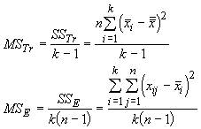
The first term is the sums of squares for the treatments (SSTr) and the second is the sums of squares for the errors (SSE). Of course, a real estimate of the variance would be divide these sums of squares by the degrees of freedom (just like we divide the sum of the squared deviations around a mean by n-1). This is a mean square, and for the treatment (MSTr) and error (MSE) the values are:

These should look similar because they are similar the two estimates of variance we calculated before to develop the F ratio:
Which is the general way to test the significance of a one-way analysis of variance. The computational formulae for these new sums of squares are:

where the degrees of freedom are N-1, k-1 and N-k, respectively. Dividing each sum of squares by its degrees of freedom gives the mean square. These formulae can be used even when sample sizes are different: the test remains the ratio of the MSTr to MSE .
Often the situations we deal with as biologists are more complex than that described by a simple one-way ANOVA. Within in treatments we often find variation that can be explained by other factors. For example, consider a problem where a researcher is interested in determining how a new pesticide affects three different species of insects. By randomly sampling three populations of the different insects, we could develop a one-way analysis of variance using time to death as a response variable. However, what if each population had a different age structure, with some containing more old individuals than others? This would confound our results because old individuals die in a shorter time than young individuals, even without treatment by a pesticide. Such a situation would inflate the error sums of squares and make it potentially difficult to detect a significant difference among the treatments. To avoid such a problem, we would want to have equal numbers of each age class in each treatment, and this becomes a two-way ANOVA. We call the new sampling scheme blocking, and each age class represents a block within a treatment. This minimizes extraneous variation within treatments so that the variation among them can be tested.
Now we must concern ourselves with the means of each cell in the experiment. If the null hypothesis is correct then there will be a single mean (m) that describes each cell. Variation among treatments (a) and blocks (b) will result in departures from this mean such that the mean of each cell is given by:
| Blocks (b) | |||
| Treatment (a) | Nymphs | Larvae | Adults |
| Pesticide 1 | m+a1+b1 | m+a1+b2 | m+a1+b3 |
| Pesticide 2 | m+a2+b1 | m+a2+b2 | m+a2+b3 |
| Pesiticide 3 | m+a3+b1 | m+a3+b2 | m+a3+b3 |
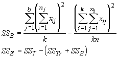
When there is no difference among treatments, then a1 = a2 = ... an = 0. When there is no difference among blocks, then b1 = b2 = ... bn = 0. Thus, if the null hypothesis is true, we expect the above conditions to also be true. We can now test the effects of treatments or blocks by testing the new parameters a and b. We calculate the SSTr just as we did for the one-way ANOVA, and the sums of squares for the blocks are given by:

where b is the number of blocks. Assuming there is no interaction between the treatments and blocks, we can use the following table to test for differences among treatments and blocks.
|
|
|
|
|
|
|
|
|
|
|
|
|
|
|
|
|
|
|
|
|
|
|
|
|
|
|
|