
Coefficient of Correlation
Statistical Inference
Partial Correlation
Coefficient
Curve Fitting
Method of Least Squares
Regression Analysis:
Regression Coefficients
Mean Value of Predictors
Limits of Prediction
Often in biology, we must deal with the association of two variables. Typically, we have an independent variable and a dependent variable. For example, we may say that body mass depends upon age, in which mass is the dependent variable. When presented with such a situation, it is often useful to determine how much of the variation in the dependent variable can be explained by the association between both variables. To examine this type of variation, we use correlation analysis.
Both the independent variable and dependent variable have variances associated with them. Just like in algebra (remember algebra?) we use x to represent the independent variable and y to represent the dependent variable. To find the variance, we would sum the squared deviations of the variables from their mean and then divide by the sample size minus 1. For correlation analysis, we will concentrate on the sums of squares, and not use the variances (or mean square). The sums of squares for the dependent variable is given by:

and for the independent variable by:

These quantities tell something about how each variable varies, but they tell us nothing about how they covary. The degree to which they covary is called the covariance, which is given by:

which is also the mean of sum, but not the sum of squares. Instead, this is the sum of the cross products

With these three statistics, we can determine the proportion of variation in y explained by the association between x and y. We call this new statistic the coefficient of determination, and it is given by:

Sometimes it is useful to know if the relationship is positive (increasing y with increasing x) or negative (decreasing y with increasing x). This is accomplished by calculating the coefficient of correlation
So, the coefficient of determination is the square of the coefficient of correlation. Because these formulae use the cross product, this is often called the product-moment correlation.
When r is either -1 or 1, then all the variation in the Ys can be explained by their association with the Xs. Conversely, when r is zero, then none of the variation in the dependent variables can be explained by their association with the independent variable. In most real world situations, however, the correlation coefficient is rarely exactly 0 or +/- 1. Rather, it is a continuous variable between -1 and 1.
When interpreting the correlation between variables, we must exercise some caution. First, it is assumed that any relationship between the variables is linear. Second, this analysis is very sensitive to "outliers". Outliers are values that deviate widely from the linear association, and these can have a large effect. It is always a good idea to plot the values for x and y against each other beforehand to determine if either of these conditions exist.
As with the other statistics we have calculated, the correlation coefficient has a confidence interval. To estimate this interval, we must assume that the independent variables have a normal distribution. With that assumption, we can transform the correlation coefficient using Fisher's Z transformation.
Which closely approximates a normal distribution, with:

and where r (rho) is the correlation coefficient of the population. The confidence interval for the correlation coefficient of the population is given by:
Given this, we can determine if the sample correlation coefficient is significantly different from a given population value by first transforming the population parameter and sample statistic using Fisher's Z transformation and then standardizing the values to get the test statistic:
For example, if we suspect that the correlation between hindleg and total length of lizards was 0.8, we could collect a sample to test this hypothesis. Below are the values for 10 lizards
|
|
|
|
|
|
|
|
|
|
|
|
|
|
|
|
|
|
|
|
|
|
|
|
|
|
|
|
|
|
|
|
|
|
|
|
|
|
|
|
|
|
|
|
|
|
|
|
|
|
|
|
|
|
|
|
|
|
|
|
|
|
|
|
|
|
|
|
|
|
|
|
|
|
|
|
|
|
|
|
|
|
|
|
SSx = 7.536; SSy = 0.549; Sxy = 1.758; r = 0.846.
Next, we must transform our hypothesize and observed correlation coefficients:

The test statistic is given by:
Using an a of 0.05, the critical values of z are -1.96 and 1.96. Thus, we fail to reject the hypothesis that the correlation between total length and hindleg is 0.80.
When sample sizes are large (>35), the correlation coefficient has a sampling distribution that can be approximated by the t-distribution with n-2 degrees of freedom. The test statistic:
can be used to determine if there is a significant correlation between the variables (H0: r = 0)
Sometimes, we may have more than two variables that may be interrelated. This most often arises when we feel that a third variable my also influence the dependent variable. In those cases, we would like to remove the effect of the third variable, and this is accomplished with the partial correlation coefficient. For the case of three variables, there are three correlations (3C2 = 3), namely rxy, rxz, and ryz. The association between variables x and y, removing the effect of z, is given by:
As we have seen, there are cases when biologists are interested in the association between two sets of paired observations. When such an association exists, it is often useful to be able to make predictions about one (dependent) variable based on the other (independent) variable. To accomplish this, we must represent the association mathematically. We call the mathematical expression that accomplishes this a curve, and we are attempting to fit the best curve to our data.
Curves can be both linear and nonlinear. Probably the simplest way to determine the appropriate curve is to examine a plot of the data. In the figure below, there are two dependent variables (blue and red) associated with a single independent variable (x).
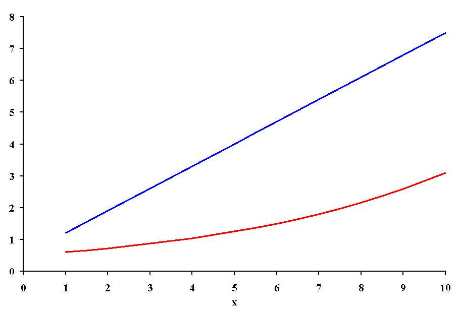
One of these data sets (blue vs x) is fairly well described by a straight line. The equation for a straight line (remember algebra?) is:
In the second data set (red vs x) the association is obviously not linear. In fact this is similar to the allometric relationship seen for the rates of many biological processes when compared to body size. The equation for an allometric relationship is:
Of course, this is a subjective means of determining the curve that best describes a set of data. There are more objective means, but their implementation is beyond the objectives of this course. In this class, we will use our intuition about biological relationships to determine the best curve for a given problem.
Knowing which curve best represents the data is only part of the problem. We would also like to know the parameters for the unknown values. For a linear equation, we would like to know what the intercept (a) and slope (b) are. These are our regression coefficients, and we must estimate them from the observations. Unfortunately, our observations rarely fall on a straight line. We can build on the procedures developed in determining correlations, however, to get an estimate of the regression coefficients.
One way to determine which regression coefficients best fit
the data (given a particular curve) is the method of least
squares. With this method, the regression coefficients that
produce a curve that minimizes the squared differences between
the data and the predicted points on the line are used to estimate
the best fit. The curve based on these regression coefficients
is the least-squares curve. We call the value of y,
for a given value of x, which falls on the least-squares
curve the predicted value ![]() , and
the method of least squares seeks to minimize the sum of all the
squared differences between the observed values of y and
the predicted values:
, and
the method of least squares seeks to minimize the sum of all the
squared differences between the observed values of y and
the predicted values:

For linear equations, this is a fairly straightforward problem, so we shall concentrate on linear regression for now.
The solution for the condition of minimized least squares is fairly complicated. One can produce two normal equations, using calculus or algebra, which hold when the least squares are at their minimum value:
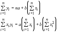
Once the various sums are calculated, then one can use Gaussian elimination to solve for the regression coefficients. As an example, let use the number of fruits set by a plants at different ages.
|
|
|
|
|
|
|
|
|
|
|
|
|
|
|
|
|
|
|
|
|
|
|
|
|
|
|
|
|
|
|
|
|
|
|
|
|
|
|
|
|
|
|
|
|
|
|
|
|
|
|
|
|
|
|
|
|
|
|
|
Substituting the sums into the normal equations, we get:
If we solve the first equation for the intercept, we get:
Substituting this value into the second normal equation we can solve for the slope:
Now, we can substitute our value for the slope into the first normal equation and determine the intercept (a = 31.533).
As you have probably guessed, there is a simpler way of doing this. In our discussion of correlations we introduced some new measures of dispersion, the sums of squares and the sums of the cross products. To review, the equations were:


We can use these and the sample means to determine the regression coefficients:

To demonstrate the use of the sums of squares method we will use the plant data again.
|
|
|
|
|
|
|
|
|
|
|
|
|
|
|
|
|
|
|
|
|
|
|
|
|
|
|
|
|
|
|
|
|
|
|
|
|
|
|
|
|
|
|
|
|
|
|
|
|
|
|
|
|
|
|
|
|
|
|
|
|
|
|
|
|
|
|
|
|
|
|
|
The necessary values are:
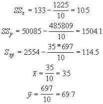
With these values we get b = 10.905 and a = 31.533, exactly the same as with Gaussian elimination. Now that we have all the necessary coefficients, we can produce the linear regression equation for our plants:
and compare it to the observed values.
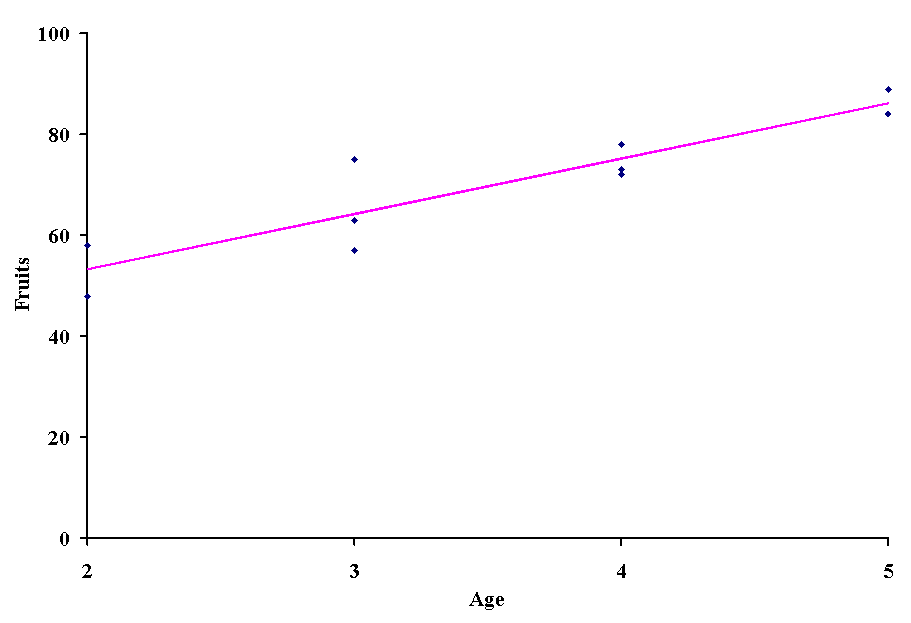
None of the actual observations fall on the regression line, but in general the line splits the difference between the highest and lowest values for any given age. The predicted values can be viewed as the average number of fruits for a given age. You probably see where this is taking us: we can make inferences about the slope, intercept and predicted values of a regression.
There are three types of hypotheses (questions) that one can address with regression analysis.
- Is the model a good indicator of the true relationship between the variables? This basically asks how confident we can be in a and b.
- Is the predicted value for a give x a good estimate of the true value?
- In what range of values do we expect ys to fall for a given x and a level of confidence?
We will discuss each of these in turn.
The slope (b) and intercept (a) are only estimates of the real quantities (b and a, respectively) in a population. The true regression equation can be represented by:
In this case yi is the mean of a sampling distribution of values for a given value of xi. From this, we can proceed as we have for all our other analyses: determine the critical test value for the sampling distribution and the standard error of the estimator. Unfortunately, the sampling distribution may not always be the same. By convention, we assume that it is normal. This allows us to simplify the process of developing test statistics, but it has the disadvantage that departures from normality can lead us astray.
Based on the assumption of normality, we can use the standard errors for our regression coefficients to develop test statistics.
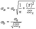
This introduces a new parameter, the standard error of the estimate (se). It is a measure of the deviations of predicted values for observed values:
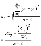
The sampling distribution is best approximated with a t-distribution having n-2 degrees of freedom. For the intercept the test statistic is:

and for the slope it is:

Using the plant data again, we get se = 5.65 and the test statistic for the intercept is:

Typically, we test the intercept for difference from zero. If it is not significantly different from zero, then it is safe to regress through the origin. One often has a relationship for which it is reasonable to expect the curve to go through zero (say size vs age or response vs drug dose). By testing the intercept, we can determine if the sample produced the desired result. For the plant data, when we test the null hypothesis that the intercept is zero, we get the test statistic t = 4.96. This is greater than the critical value with 8 d.f. and 95% confidence. It would appear our plants produce fruits even when they are aged zero!
We can also test the null hypothesis that the slope is zero. A slope of zero means that values of y are unrelated to values of x (similar to testing the correlation coefficients).
which is also significant with 8 d.f. If both the slope and the correlation coefficient are an indication relationship between the variables, do we not expect the correlation coefficient to be significantly different from zero as well?

In fact, they are both a test of the same hypothesis (just worded differently). Of course, there are situations where the hypotheses may be different. We may want to know if the slope equals a particular value (e.g., b = 20.5). In this case the null hypothesis may be false, but the correlation will still exist.
Now, we turn to the second question addressed with regression analysis. How confident are we that the predicted value of y for a given x is the mean of the population for that value of x? This is simply an extension of the last question, and the test statistic is given by:

If this looks similar to the test for the intercept, that is because it is. The intercept is the mean for a particular value of x, when it equals zero. One can test the null hypothesis that a given predicted value equals 0 or some hypothesized value for each value of x. More commonly, this relationship is used to determine the confidence interval around each predicted value.

It is often tempting to extrapolate regression analysis to observations that don't exist in the data used to produce them. This is generally a dangerous proposition, however, we can produce confidence limits for a value beyond the data with the following equations:

Although the maximum age of the plants sampled was 5, we can produce a confidence interval for age 7 in which we are 95% sure the real value of fruits will be found.

This means the number of fruits set at age 7 is between 88.25 and 127.49. If you can live with that margin of error, then you may feel comfortable making predictions about the plants when they are 7.