11 Nonlinear and Multiple Regression

Topics

Nonlinear Regression Analyses:

Exponential Functions
Power Functions

Limits of Prediction
Multiple Regression Analyses

Linear Functions
Nonlinear Functions
Limits of Prediction

Nonlinear Regression Analyses

As we said before, linear regression methods only apply to straight-line relationships between the variables. Often in biology, we encounter variables that are related in a nonlinear fashion. We can apply these techniques by forcing the relationship to be linear in some scale. This is accomplished in different ways, depending upon the type of hypothesized relationship. We will explore only a few here.

Exponential Functions

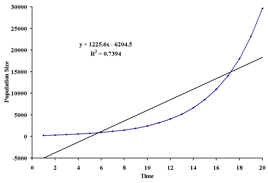
In many situations, the relationship between variables takes the shape of an exponential function. This means that the ys increase or decrease more rapidly than the xs. A classic example in biology is the exponential growth of populations. If we attempt to fit a straight line through the points, we come up with some useless results, as exemplified with the following figure:

Although all of the points fall on a smooth curve, the proportion of the variation in population sizes that can be accounted for by the straight line is only 74%. Worse still, the straight line predicts an intercept of -6204.5 which means that the population started with a negative number of individuals, which of course is impossible.

The equation for exponential growth is:

where N_t is the population size at some time (t), N₀ is the starting population size (intercept) and r is the intrinsic rate of increase. How can we make this linear? If we take the log of each side we get the following equation:

Now we can let y = ln(N_t), a = ln(N₀), b = r and t = x to get the typical linear regression equation, y = a + bx. If we plot the log of N against time, we iget a straight line.

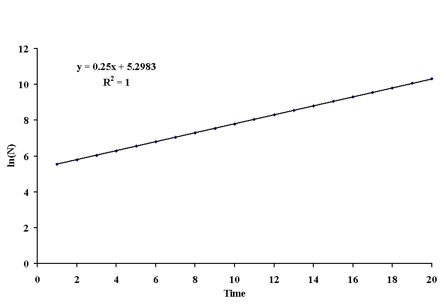
With this type of transformation, b is the intrinsic rate of population increase (0.25), and a is the log of the starting population size (e^a = e^5.2983 = 200). For this particular population, we can predict future population sizes with the following equation:

To find the least squares equation for such data, we proceed just as with linear regression, except all the ys are ln(N). A table for calculating the regression coefficients follows:

Giving us:

This is obviously a better fit to the data (r = 1.00), and the intercept yields a positive number for starting population size instead of a negative. Of course, we test the significance of these regression coefficients using a and b, not the starting population size and the intrinsic rate of increase.

Power Functions

In some cases, the dependent variable is a power function of the independent variable. An excellent example from biology is the allometric equation. This equation relates the rate of a physiological function to body size, and it looks like:

where s is the allometric scale and c is the allometric constant. An example is the relationship between body size and metabolic rate in homeotherms.

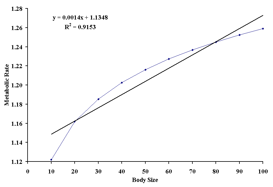
Obviously, the straight line doesn't fit the points very well. Although the coefficient of determination is very high, all of the points actually fit on a smooth curve which better explains the variation in ys. Also note the intercept is 1.13, which suggests that even animals with no size have a metabolic rate, which we know is impossible. There are actually two ways to approach this problem.

Remembering back to the example we used for fruit set in plants, we found an intercept that was greater than zero. This suggested that plants of age zero still produced fruits: again this is impossible. However, over the range of ages we obtained the relationship was fairly linear. As long as we confined our predictions to this range of ages, we could be fairly confident in them, but extrapolating outside that range increased our probability of making an erroneous prediction. This is the problem with regression when it is used to predict values for which we have no supporting data. Note that in the example for metabolic rate, the relationship is fairly linear for large body sizes. We may be satisfied with limiting our analysis to that range of the data and ignoring the lower body sizes and metabolic rates. In such a case, we would proceed with a normal linear regression model. This simplification, however, ignores an important consideration. We may have a theoretical reason to expect a certain nonlinear relationship to occur between to variables (perhaps because such a functional response has appeared in similar studies). In such cases, it would be a mistake to ignore the underlying biological mechanism merely to simplify our model: we may miss important insights about our data.

We would like to use all the data (usually a much better approach), so we must linearize the relationship in some fashion. Again, we can take the log of our ys to produce a linear relationship. In this case the equation is:

Now we proceed just as we did with exponential regression except that we must also use ln(size) to represent x..

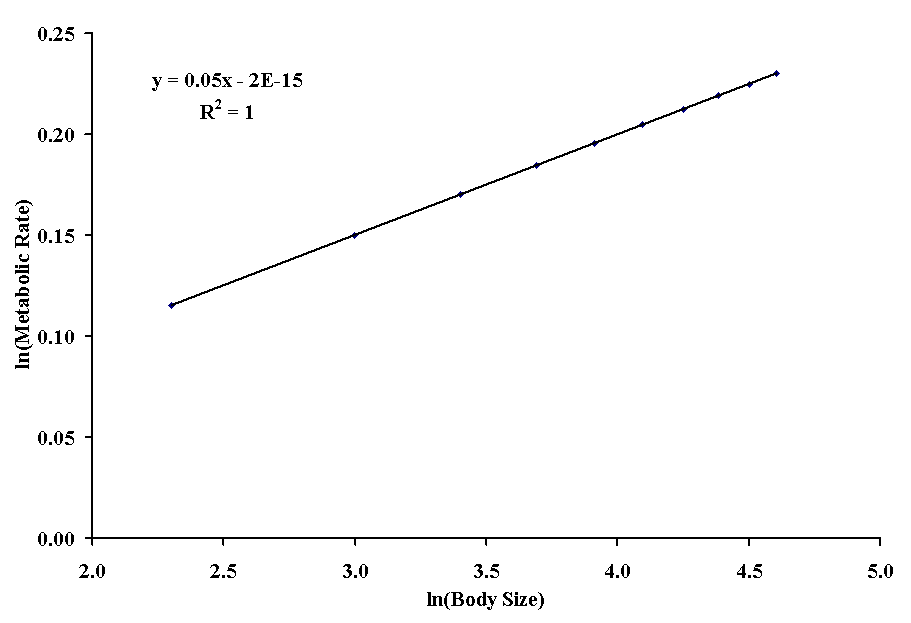
Note that we now have a slope of 0.05, which is the allometric constant. The intercept is very close to zero (just a small rounding error, it will never actually reach zero on a log scale!), which is as it should be. To find the allometric scale, we simply find the exponent e^a = 1.00. The following table shows the calculation of the regression coefficients for this problem.

Multiple Regression Analyses

Often, we find that variation in our independent variable is poorly explained by a single independent variable. For example, we may regress body size against age and get only a moderate fit (e.g., r = 0.32). Intuitively, we realize there are many things that can influence body size, like sex (if the species is sexually size dimorphic like humans), genetics (e.g., if the parents were large), and environment (e.g., if a variable amount of food was consumed during development). We could do four separate regressions, but as we saw in the discussion of correlations, these independent variables may be correlated with each other. Simply summing the coefficients of determination for each separate regression will not tell us how much variation are explained by all the independent variables. Further, we will have no way of determining a single intercept and slope. The better approach is to simultaneously fit the dependent variable to all independent variables, again minimizing the squared difference between the observed and predicted values. We call this approach multiple regression.

Linear Functions

If the dependent variable is linearly related to each of the independent variables, then we can extend our linear equation to account for them:

In this case, each independent variable has a different slope associated with it, but there is still only a single intercept. As with our previous linear models we proceed from a set of normal equations, which look like the following for two independent variables:

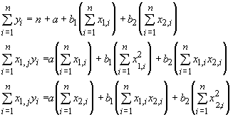
From these we can solve, with Gaussian elimination, for each of the regression coefficients. As with simple linear regression, there are formulae for the regression equations that involve sums of squares and sums of cross products. Before we examine these formulae, we must introduce some new statistics. They are:

With these, the regression coefficients can be found with:

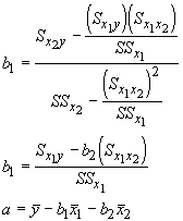
By simply producing a table as we have will all the regression problems, we can easily find the coefficients. Now let's use our body size problem again. For several ages, we have the size of a lizard and their food intake.

The values necessary for calculation of the regression coefficients are:

In order to determine the amount of variation in size that can be accounted for with these two independent variables, we can proceed as we did for multiple correlation. This can be a tedious undertaking with several independent variables. A better way is to use the ratio of two sums of squares, which requires us to define a few new terms. In the process of performing a regression, we have accounted for a portion of the total variation in ys with our predicted values. When the fit is not perfect,we have some residual variation that is not accounted for. We can define three sums of squares for these three aspects of variation. The sums of squares for total variation (SS_tot) in ys we have already seen as SS_y. The sums of squares for the regression (SS_reg)compares the predicted values to the mean value of the ys. The sums of squares of the residuals (SS_res) is the comparison of the predicted to observed values.

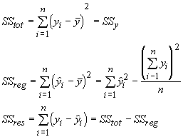
The multiple correlation coefficient is given by:

For this particular regression, we have an r of 0.89. We will expand on these methods when we explore analysis of variance next week.

Nonlinear Functions

Nonlinear relationships can also exist when there are curvilinear relationships that cannot be explained by exponential or power functions. If there are changes in the direction of y given a range of xs, then we are probably dealing with a polynomial function. It is a simple matter to fit polynomial relationships between an independent variable and a dependent variable with multiple regression. The polynomial function is given by:

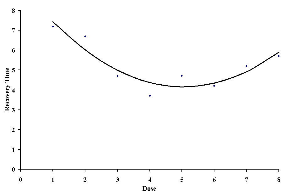
This representation is a linear equation, we simply raise values of x to different powers. The most simple form of this relationship is the parabola. One might see a parabolic relationship when dealing with may types of data. As an example we will use recovery time in response to doses of a new drug.

which yields:

These quantities give us a regression equation of y = 9.24 - 2.01x + 0.20x². This equation produces a correlation coefficient of 0.85, and as you can see, it is a pretty good fit to the original data.

A word of caution: with a long enough expression (i.e., k = n - 1), we can fit a curve through every observation of y. Generally, third order (k = 3) or above fits should be looked upon with skepticism in biological data, as these indicate higher-order intereactions between variables that only rarely have a good theoretical explanation.

< Go back to Topic 10                         Go on to Topic 12>