Full Factorial Designs
Fractional
Factorial Designs
Central Composite Design
Experiments are often made to determine the relationship between a response to some set of variables of interest, usually by constructing a model that describes the response over an appropriate range of these variables. These models may be referred to as response surfaces, in that the response can be graphed as a two-dimensional curve (with one variable) or as a three- or more dimensional surface (with two or more variables). These surfaces can in turn be used in characterizing the response for descriptive or optimization purposes. Empirical functions of the form:
may be derived, where y is the response and x1, x2, x3, ..., xk are quantitative levels of the factors of interest. A response surface can have an infinite number of possible shapes, depending upon the response function's shape as determined by a fitted model. Experiments with only two factor levels per variable (m = 2) are therefore limited, in that only linear functions of the variables can be fitted to the response. Unless the response is known to change linearly with changes in all of the variables, it is generally desirable to use at least three levels for each variable in the experiment. This permits quadratic functions of the variables to be used in estimating the response, which is especially important if the response shifts abruptly with a slight change in one or more of the variables. Repeat tests are also included to provide information on the experimental-error variation.
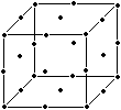
Fractional Factorial Designs The mk factorial can be conceptually represented using a 'factor space': a k (where k = the number of variables) dimensional hypervolume where m treatment levels (factors) are arrayed at equal distances along each dimensional axis. Because such designs rapidly become very large as the number of variables increases (see below), they are most useful in initial explorations of the factor space to identify the region of optimal response. For example, the treatment combinations for a full factorial design with three variables (1, 2 and 3) at three levels (-1, 0, and 1) per variable (33 = 27 treatment combinations) can be described as a cube:

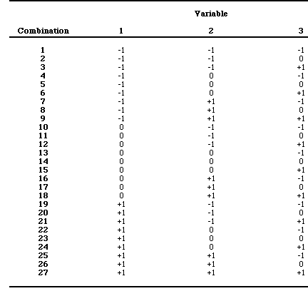
where each dot corresponds to one treatment combination, i.e., 27 runs of the following combinations:

Using a design with 4 variables of three levels each, the number of runs rapidly increases to 81; for a 5 variable experiment, 243. Moreover, these designs do not give equal precision for fitted responses at factor-level combinations (points on the factor space) that are at equal distances from the center of the factor space. Designs that do have this property are termed rotatable . Rotatable designs are more desirable because the orientation of the design with respect to the response surface is unknown before data collection and fitting of the data to the surface has been accomplished. Ordinarily, repeat observations (if any) are taken at the center. If repeat observations are made at the vertices, there must be an equal number of observations made at all the design points to maintain rotatability. For more than two factors, design points should be on a sphere or hypervolume in four or more dimensions, and must form a regular geometric figure (e.g., a cube) to be rotatable. All 2k factorials are rotatable, but 3k factorials are not. There are, however, other classes of designs with 2 or more factors that can be used instead of 3k factorials to fit second-order polynomials to response surfaces.
In addition, such high numbers of runs are necessary only where there is significant higher order interaction between the variables. In many biological situations, three-way and higher order interactions may not be significant, so simplified models (e.g., fractional factorials) that address only first- and second-order interactions between the main effects.
Three designs that are more efficient than 3k factorial experiments are the face-centered central composite design, the central composite design, and the Box-Behnken design. All are fractions of 3k factorials, but only require enough observations to estimate the second-order effects of the response surface. They can also be made rotatable (or nearly so). The central composite design for three factors is illustrated below:

The Box-Behnken design is similar to the full factorial design above, except that the points on the faces and corners of the cube are removed, and midpoints are added to the center of the cube (i.e., there are points in the center of the cube, and at the center of each of the cube's edges). The face-centered central composite design, has points located at each corner of the cube, at the center of each face, and at the center of the cube (note : when overlaid, the Box-Behnken and the face-centered central composite designs collectively form a full factorial design). In certain situations where measurement errors for the variables are likely to be significant, the face-centered central composite design has the advantage of using the fewest levels (3) for each variable, whereas the other two designs require five levels (0, ±1, ±a ). I chose the central composite design for my experiment because it provides more levels for each variable than the face-centered composite design, which seemed best for examining the linearity of each of the variables, and because (unlike the Box-Behnken design) it is rotatable, yet requires only a few more runs. Furthermore, the numerical range of each of the variables is greater in the central composite design compared with the the Box-Behnken design.
The central composite design is constructed as follows (Mason et al. 1989, Ch. 11):

The total number of test runs in a central
composite design based on a complete 2k factorial is n = 2k + 2k + m . This is generally
< 3k , so fewer
observations are required than with a 3k factorial. The central composite design can be made
rotatable by choosing a = F 1/4, where
F is the number of factorial points (e.g., F
= 2k when a
complete factorial is used). In the example above, k =
3 and 23 = 8, F 1/4
= ![]() or 1.68.
or 1.68.
Example:
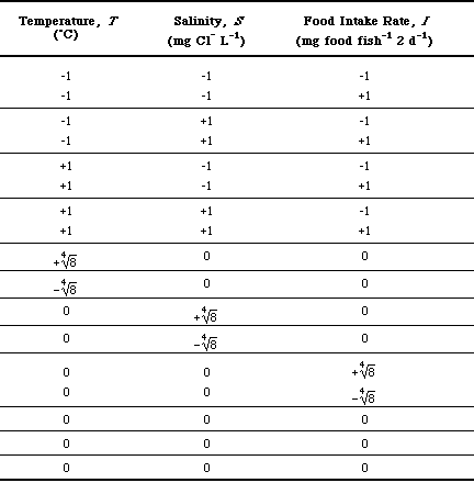
In my goldfish experiment, there are three variables:
|
|
|||||
| Variable |
|
|
|
|
|
| 1. Temperature, T (°C) |
|
|
|
|
|
| 2. Salinity, S (mg Cl - L-1) |
|
|
|
|
|
| 3. Food Intake Rate, I (mg food fish -1 2 d-1) |
|
|
|
|
|
|
|
|
|
|
|
|
|
|
|
|
|
|
|
|
|
|
|
|
|
|
|
|
|
|
|
|
|
|
|
|
|
|
|
|
|
|
|
|
|
|
|
|
|
|
|
|
|
|
|
|
|
|
|
|
|
|
|
|
|
|
|
|
|
|
|
|
|
|
|
|
|
|
|
|
|
|
|
|
|
|
|
|
|
|
|
|
|
|
|
|
|
|
|
|
|
|
|
|
|

As you can see, this produces a design with a total of 17 treatment combinations.
Mason, R.L., R.F. Gunst, and J.L. Hess. 1989. Statistical Design and Analysis of Experiments with Applications to Engineering and Science. New York. JohnWiley and Sons. 692 pp.