Tests of Randomness
Test of Central Tendency
Sign Test:
small
and large sample size
Signed Rank:
small and large
sample size
Rank Sums: Wilcoxon's Rank Sums, Mann-Whitney U, and Kolmogorov-Smirnov tests
Rank Sums (k Means): Kruskal-Wallis
H
Two-way Factorial (Friedman's test)
Oten, it is impossible or unwise to make the assumptions regarding normality that we have made for the tests previously discussed in this course. A special class of statistics have been developed for such situations. We describe the normal statistics (which we have discussed so far) as parametric because they use most of the information in the sample. Nonparametric statistics reduce the information such that samples fit some predefined distribution. In general, nonparametric statistics are easier to compute and easier to understand than parametric statistics, but they have less power than normal statistics if the data do in fact meet the assumptions of the test.
Distribution-free tests are tests whose validity under the null hypothesis does not require a specification of the population distribution(s) from which the data have been sampled.
All of the parametric methods we studied in this course assume that our samples are random, but we have developed no methods for determining randomness. Instead, we relied upon our sampling methods to produce a random sample. Determining if a sample is random is a difficult task to accomplish with parametric statistics, but it is relatively simple using nonparametric techiniques. We accomplish this we can use runs, which are a succession of identical symbols separated by different symbols. For example, we may use the letters in the alphabet or simply + and - signs. The number of runs is a good indication of randomness; if there are few runs we may suspect grouping and if there are many runs we may suspect some repeating pattern.
As an example of runs, we can use a sample of birds from an island. A previous researcher collected the sample and provided the age classes (juvenile vs. adult) for each individual. We will assign - signs to the juveniles and + signs to the adults. Below are the data, in order of collection, with our symbols for the runs:
|
|
|
|
|
|
|
|
|
|
|
|
|
|
|
|
|
|
|
|
|
|
|
|
|
|
|
|
|
|
|
|
|
|
|
|
|
|
|
|
|
|
|
|
As you can see, there are equal numbers of juveniles and adults.
The question is, does this represent a random sample of the population?
In this case we have three runs of juveniles (-) and two runs
of adults (+). There are a total of 5 minus signs (n1
= 5) and 5 plus signs (n2 = 5). The total number
of runs is 5 (u = 5). We reject the null hypothesis that
the sample is random if ![]() or
or
![]() . For our sample sizes we get
. For our sample sizes we get
![]() and
and ![]() . Because
u falls between these values, we can say this represents
a random sample (fail to reject the null hypothesis). Presumably,
there is a nearly equal distribution of adults and juveniles in
the population, and it would be safe to proceed with a test of
proportions to confirm this hypothesis.
. Because
u falls between these values, we can say this represents
a random sample (fail to reject the null hypothesis). Presumably,
there is a nearly equal distribution of adults and juveniles in
the population, and it would be safe to proceed with a test of
proportions to confirm this hypothesis.
What if the proportions of adults and juveniles were not equal? Say there are very few juveniles and many adults. It is possible that we would have found only one juvenile in our sample of 10 individuals. If that one juvenile had occurred at either end of the sampling order we would have had two runs. If it had occurred anywhere else we would have had three runs. Given sample sizes of 1 and 9, is it possible to get a result that would reject the null hypothesis of randomness? Examination of the table will show there are no critical values for this combination of sample sizes. This means that we can't reject the null hypothesis, regardless of the number of runs.
When neither sample size is less than 10, then the sampling distribution is approximately normal for the runs statistic (u). The mean and standard error are:
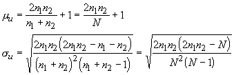
and we can use our z-statistic to test the assumption of randomness:
This is a two-tailed test, so we reject the null hypothesis
when the inequality statement ![]() is
not true.
is
not true.
When dealing with numerical data, we can approach the problem in a similar manner. We can compute the median of the sample (or use some hypothesized median for the population) and assign minus signs to values below the median and plus signs to values above. All values that are equal to the median are dropped from the data set (and not counted in the sample sizes). These symbols can then be used to determine the number of runs. For example, we have data on the distance that bees fly to find pollen on their first excursion of the day.
|
|
|
|
|
|
|
|
|
|
|
|
|
|
|
|
|
|
|
|
|
|
|
|
|
|
|
|
|
|
|
|
|
|
|
|
|
|
|
|
|
|
|
|
The median for this sample is 3.0 and we obtain 5 runs. Note now that exactly half the values fall on either side of the median, so n1 = n2 = 5. Our critical values are 2 and 10, so we can't reject the null hypothesis that this sample is random with respect to distance traveled. Of course, with large sample sizes we can use the same methods described in the last section.
In general, we view the nonparametric tests of central tendency as a test of the median, not the mean. In the case where the population distribution is normal, the median and the mean are equal. In the case of normal distributions, the following tests are testing the same hypotheses as the equivalent parametric statistics. When the population is not normal, these test are best viewed as dealing with central tendency.
For the sign test we must have a continuous population with
equal probability of getting values above and below the median.
In this case we are talking about the population median, so it
works much like the one sample t-test we discussed earlier.
We are testing the null hypothesis that ![]() , so
we assign a minus sign to sample values less than the hypothesized
median and positive signs to values above the median. Again, we
discard values that are exactly equal to the median.
, so
we assign a minus sign to sample values less than the hypothesized
median and positive signs to values above the median. Again, we
discard values that are exactly equal to the median.
As an example, let's use the same data on distance traveled
by bees. We will test the null hypothesis that ![]() vs.
the alternative that
vs.
the alternative that ![]() , so
we must change the symbols (note, order no longer matters).
, so
we must change the symbols (note, order no longer matters).
|
|
|
|
|
|
|
|
|
|
|
|
|
|
|
|
|
|
|
|
|
|
|
|
|
|
|
|
|
|
|
|
|
|
|
|
|
|
|
|
|
|
|
|
By doing this, we have reduced the problem to one of binomial probabilities. We expect half the individuals to fall on either side of the median, so P = 0.5. We have a total sample size of 10 (n), and we find 4 values above the median (x). Using a table for binomial probabilities, we see the total probability of obtaining 4 or less observations is 0.001+0.010+0.044+0.117+0.205 = 0.377, which is greater than α = 0.05. Thus, we can reject the null hypothesis that median flight distance is greater than 4.5 m.
How would one perform a two-tailed test for such a statistic? Actually, it is rather simple. Let x represent the smaller of the two groups of symbols (in this case it is still 4) and let y represent the total of the larger group of samples (6). Now, calculate the total probabilities of obtaining values less than or equal to x and greater than or equal to y. They should be identical, because the binomial distribution is symmetrical. Thus, we can use either probability to compare with α/2.
When we have paired data, then we can also use the sign test to determine if two samples are significantly different from each other. We assign plus signs to pairs that have the first value is greater then the second, and minus signs when the second value is greater than the first, and we discard ties. If the samples are truly equal, then we expect the number of plus signs to equal the number of minus signs (P = 0.5). Thus we can proceed in the same manner as described above.
As we saw in earlier lectures, when np and n(1-p) are both greater than 5 we can use the normal approximation to the binomial distribution. In such cases, we can use a z-test of the form:
The sign test does waste a lot of information because it only uses the sign. It is impossible to detect a departure from the null hypothesis with fewer than six pairs of observations. We can, however, rank the values to retain a little more information about the samples (and hopefully the populations they came from). In this test we rank the values based on the difference from the hypothesized median, ignoring the sign (i.e. -3 has a higher rank than 2). Again, zero differences are discarded. When two or more values are tied we take the median rank of their values. From these values we can sum the ranks for negative values (T-) and positive values (T+).
As an example of the signed rank, we will use our bees again
and test the null hypothesis ![]() against
the alternative that
against
the alternative that ![]() . We
subtract the hypothesized value from the real values to get the
signs, and then rank the values:
. We
subtract the hypothesized value from the real values to get the
signs, and then rank the values:
|
|
|
|
|
|
|
|
|
|
|
|
|
|
|
|
|
|
|
|
|
|
|
|
|
|
|
|
|
|
|
|
|
|
|
|
|
|
|
|
|
|
|
|
|
|
|
|
|
|
|
|
|
|
|
The sum of the positive ranks is T+ = 8+2+10+3.5 = 23.5, and the sum of the negative ranks is T- = 1+6.5+3.5+6.5+5+9 = 31.5. We define a statistic T which is the smaller of T+ and T- (in this case 23.5). To test various hypotheses we must use different criteria:
|
|
|
|
|
|
|
|
|
|
|
|
|
|
|
|
In this case, we are using the first type of test, so we would reject the null hypothesis if T+ is less than or equal to the critical value for 2*0.05. In this case, the critical value is 11, which is less than our calculated value. Therefore, we can't reject the null hypothesis that median flight distance is 4.5. Why did we get a different result from that when we used the sign test? We have retained more information, and with that extra information, we have lowered the probability of rejecting the null hypothesis when it is true. Thus, the signed rank test has more power than the sign test alone. When dealing with numerical data is preferable to use the signed rank test.
As you have probably guessed, we can use the signed rank for paired data as well. We simply use the difference between the two samples and ranks these values.
When n is about 15 or larger, then the T statistic has an approximately normal distribution with:
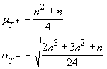
and one can use the z-test

to determine significance.
The Wilcoxon one-sample signed rank test is used to test the null hypothesis that the median of the population from which the data sample is drawn is equal to a hypothesized value. It is equivalent to a one-sample t-test (except that the median, rather than the mean, of the sample is tested against an expected value, e.g., 0), but does not assume normality.
The Wilcoxon two-sample paired signed rank test is used to test the null hypothesis that the population median of the paired differences of the two samples is 0.
This test assumes that:
Because the test statistic for the Wilcoxon signed rank is based only on the ranks of the paired differences, the test can be performed when the only data available are those relative ranks for the paired differences. Note that it is not assumed that the two samples are independent of each other. In fact, they should be related to each other such that they create pairs of data points, such as the measurements on two matched people in a case/control study, or before- and after-treatment measurements on the same person.
The two-sample paired signed rank test is equivalent to performing a one-sample signed rank test on the paired differences.
While the previous nonparametric statistics for two samples could be applied to either tests of a single median or test of two medians with paired data, they cannot be applied to tests concerning unpaired data. For this we can use the Wilcoxon's Rank Sums test, or the Mann-Whitney U test (which is equivalent to the Wilcoxon rank sum test, but can deal with unequal sample sizes). These rank sum tests are used to test the null hypothesis that the two population distribution functions corresponding to the two random samples are identical against the alternative hypothesis that they differ by location (location is the generalized "average" value of a distribution, e.g., the mean, the median, the mode, and the geometric mean). Another test, the Kolmogorov-Smirnov two-sample test, tests whether two independent samples come from identical distributions (either continuous or discrete). For example, it can be used to test whether a sample data set has a normal (or any other) distribution by comparing the data values against an expected normal distribution that is assumed to have the same mean and variance as the sample data. The Kolmogorov-Smirnov test is considered to be conservative, because the probability of a Type I error is less than the specified a-value.
This test assumes that:
Within each sample, the values are independent, and identically distributed. (we need not specify or know what the distribution is, only that all the values in each sample follow the same continuous distribution).
The two samples are independent of each other.
The populations from which the two samples were taken differ only in location. That is, the populations may differ in their means or medians, but not in their dispersions or distributional shape (such as skewness).
Because the test statistic for the Wilcoxon rank sum test test is based only on the ranks of the data values, the test can be performed when the only data available are those relative ranks. We assume that both samples are independent and come from continuous populations. To perform this test, we rank all the values (regardless of which group they belong to), and the actual test is based on the sum of the ranks. Ties are assigned the median of their ranks. When there is a large difference in the medians, then one sample will have a low sum of the ranks and the other will have a large sum of the ranks. The sum of the two ranks are denoted W1 and W2, respectively.
As an example, lets now consider two hives of bees with the following distances traveled:
|
|
|
|
|
|
|
|
|
|
|
|
|
|
|
|
|
|
|
|
|
|
|
|
|
|
|
|
|
|
|
|
|
|
|
|
|
|
|
|
|
|
|
|
|
|
|
|
|
|
|
|
|
The sum of the ranks for the first hive (W1) is 88 and for the second hive (W2) it is 102. Note that the second sample is smaller than the first (9 vs. 10 observations) so we should expect its sum to be biased downward. We must take into account sample size when performing the test, so our test values are:
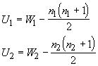
and U is the smaller of the two values. To test different hypotheses about the population median(s) we must use a table to find the critical values. The rejection criteria are given below:
|
|
|
|
|
|
|
|
|
|
|
|
|
|
|
|
For our example, we get U1 = 33 and U2 = 57. To test the null hypothesis that the central tendency is the same for both samples, we would compare the smaller (33) to the value in the table for a = 0.05. In this case the critical value is 20, and our test value is greater than that. We can't safely reject the null hypothesis that the two samples have equal central tendency.
We can use the small sample test regardless of sample size, but when sample sizes are large (both greater than 8) then the U statistic has an approximately normal distribution with:
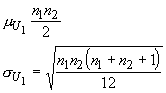
and we can use a z-test. The z-statistic is given by:

Of course, we can run into situations where there are multiple unpaired random samples that need to be tested. For a parametric test, we used a one-way ANOVA. The nonparametric equivalent is the Kruskal-Wallis H test. The Kruskal-Wallis test is used to test the null hypothesis that multiple population distribution functions (corresponding to multiple samples) are identical against the alternative hypothesis that they differ by location (for two samples, the Kruskal-Wallis test is equivalent to the two-sample rank-sum test.)
The assumptions of the Kruskal-Wallis test are:
Because the test statistic for the Kruskal-Wallis test is based only on the ranks of the data values, the test can be performed when the only data available are those relative ranks.
The data are again ranked jointly, and the sum of the ranks (Ri) are calculated for each sample. As an example, lets add a third hive of bees to our samples:
|
|
|
|
|
|
|
|
|
|
|
|
|
|
|
|
|
|
|
|
|
|
|
|
|
|
|
|
|
|
|
|
|
|
|
|
|
|
|
|
|
|
|
|
|
|
|
|
|
|
|
|
|
|
|
|
|
|
|
|
|
||
|
|
|
|
|
||
|
|
|
The sum of the ranks are: R1 = 118.5, R2 = 144, and R3 = 88.5. The H-statistic is calculated from the following equation:
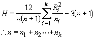
Given each sample size is at least 5, then H has approximately a χ2 distribution with k-1 degrees of freedom. For our example we get H = 7.51. The critical value from the χ2 table (with 2 degrees of freedom, α= 0.05) is 5.99. Because our test statistic exceeds this value, we can reject the null hypothesis that all the sample medians are the same.
The most commonly-used nonparametric equivalent to the two-way factorial ANOVA is Friedman's test. Friedman's test is used to test the null hypothesis that several treatment effects or locations are equal for data in a two-way layout.
Friedman's test is designed for the case of no replications (i.e., exactly one measurement at each possible combination of values for the two factor levels). When there are replications, the values in each cell (each combination of factor level values) are replaced with their mean or median (obviously, this sacrifices degrees of freedom). For example, if the 5 measured replicated values in the cell for factor 1 (Treatment) equal to "Pesticide 1" and factor 2 (Block) equal to "Nymphs" are 28, 30, 31, 40, and 50, they could be replaced with the single value 31 (the cell median).
Although Friedman's test does not assume normality of the distributions for the factor populations, it does assume that the populations have the same distribution, except for a possible difference in the population medians. Thus, Friedman's test will not address the problem of inequality of variances. Also, as with the two-factor factorial ANOVA, it is assumed that the measurement errors are identically distributed and independent of each other. In addition, Friedman's test assumes that there is no interaction between blocks and treatments.
The process of ranking values can also be applied to the problem of association between variables. One can calculate a Spearman's rank-correlation coefficient (rs) by ranking the x and y variables independently. We then calculate the sum of the squared differences between the ranks. As an example, let's use the first hive of bees, and use the time (in minutes since dawn) the bee left the hive as the independent variable:
|
|
|
|
|
|
|
|
|
|
|
|
|
|
|
|
|
|
|
|
|
|
|
|
|
|
|
|
|
|
|
|
|
|
|
|
|
|
|
|
|
|
|
|
|
|
|
|
|
|
|
|
|
|
|
|
|
|
|
|
|
|
|
|
|
|
|
|
|
If we let D represent the sum of the squared differences (178.5), then the rank correlation is given by:
For our example, the rank correlation is -0.08. To determine if this is significantly different from zero, we must perform a z-test. The standard error of rs is:
and our test statistic becomes:
Because this falls in the range from -1.96 and 1.96 (the critical values of z) we can't reject the null hypothesis that the correlation is zero.
There are other nonparametric tests, including nonparametric regressions analyses, but they are beyond the scope of this course.